“Can you improve the algorithm that classifies drugs based on their biological activity?”

About

The goal of this blog post is to describe a medal winning solution to the MoA competition on Kaggle. Since this was my first ranked competition on Kaggle and I am not a Data Scientist expert I would say that this blog post is going to be most suitable for beginners in this domain.

While describing the solution, my idea is to focus more on the overall concepts rather than going into details of the code. All of the solution code was implemented in Python, if you are only interested in the code you can find it on the github repo.

Competition explanation

The MoA abbreviation in the title of the competition stands for Mechanisms of Action. I do not have any domain knowledge for this competition, so here are some definitions that I took from the competition page where they describe some of the terms needed in order to understand the data better.

What is the Mechanism of Action (MoA) of a drug?

“In the past, scientists derived drugs from natural products or were inspired by traditional remedies. Very common drugs, such as paracetamol, known in the US as acetaminophen, were put into clinical use decades before the biological mechanisms driving their pharmacological activities were understood. Today, with the advent of more powerful technologies, drug discovery has changed from the serendipitous approaches of the past to a more targeted model based on an understanding of the underlying biological mechanism of a disease. In this new framework, scientists seek to identify a protein target associated with a disease and develop a molecule that can modulate that protein target. As a shorthand to describe the biological activity of a given molecule, scientists assign a label referred to as mechanism-of-action or MoA for short.”

How do we determine the MoAs of a new drug?

“One approach is to treat a sample of human cells with the drug and then analyze the cellular responses with algorithms that search for similarity to known patterns in large genomic databases, such as libraries of gene expression or cell viability patterns of drugs with known MoAs.

In this competition, you will have access to a unique dataset that combines gene expression and cell viability data. The data is based on a new technology that measures simultaneously (within the same samples) human cells’ responses to drugs in a pool of 100 different cell types (thus solving the problem of identifying ex-ante, which cell types are better suited for a given drug). In addition, you will have access to MoA annotations for more than 5,000 drugs in this dataset. Note that since drugs can have multiple MoA annotations, the task is formally a multi-label classification problem.”

In more concrete terms we have training data that contains 23 814 rows where each row has 876 columns. Each row represents a single sample in the experiments and it is associated with a unique identifier sig_id. Additionaly, we have a target dataset that contains 23 814 rows and 207 columns where 1 column is for the sig_id while the other 206 are representing the unique MoA targets. So, for every sample in the training data we have associated target vector in the target dataset that represents which MoAs are activated given the sample gene expressions and cell viability. Our solutions are scored on a new test dataset that contains around 12 000 rows with the same 876 feature columns and we need to predict the activated MoAs for every sample in this dataset.

This competition belongs to the “Code competition” class of the possible Kaggle competition types. For this competition your solution must finish under 2 hours if it runs on GPU or under 9 hours if it runs on CPU. While the competition lasted, our solutions were evaluated on 25% of the test data which is known as public leaderboard. When the competition officially ends they are evaluated on the rest of the test data and we get the final standings which are known as private leaderboard. What is really interesting and challenging in the final days of the competition is that you can select only 2 solutions that will be scored on the private leaderboard. So, you need to be careful to not overfit the public leaderboard and select models the generalize the best on new data. This was tricky for me because I had submitted over 150 solutions and I had to choose only 2, but I managed to make a good selection and after revealing the private leaderboard I jumped over 850 positions.

If you are interested in reading more of the competition insights here is a really nice discussion that explains some of the things in more details and if you are more interested in deep exploratory data analysis here is a nice notebook that does that .

Defining the problem

Let’s have two variables X and Y and a function S(X) → Y. The variable X represents an input feature vector for the problem which is just an array of float numbers while the target vector Y is just an array of numbers where each number is between 0 or 1. We need to find implementation for the solution function S that for a given arbitrary input vector X_i it will provide us output vector Y_i that we think the best describes the given input X_i.

But what it means to best describe the given input ?

For a given input vector X we don’t know the true output Y_true so the best thing we can do is to come up with an approximation of it. We can call our approximated output Y_pred where we obtain it from passing X in the solution function S. On the other hand, the organizers of this competition know the true output for every input vector so they define a loss function L(Y_true, Y_pred) → V where the value V is just a float number that represents how far is our Y_pred approximation from the true value Y_true. The oraganizers want us to predict values as close as possible to the true ones, so the goal of this competition is to minimize this loss function L. When we rewrite what we have said before, for a given input X we need to find a solution function S that minimizes the loss function L(Y_true, S(X)) → V.

In order to find a good approximation function, the organizers have provided us with a train dataset D_train which is a list of train examples where each example is represented as tuple (X, Y). With this dataset at hand we need to find good use of it in order to improve our soulution function S that we have defined before. Additionaly, there is a test dataset D_test where the true Y values are hidden from us. We need to approximate those values using our solution function. In the end our score is calculated by summing up the values of the loss function L for every sample in the test dataset.

As you might have guessed by now, the input vector X will be a subset of the 876 columns given in each sample in the training data. I say subset because we are not going to use all of the features that are given to us. The predicted output vector Y_pred will be the the probability vector over the MoAs activation meaning that the i^-th element in this vector represents the probability of the i^-th MoA being activated. The competition loss function L is the mean columnwise log loss.

Solution overview

In this competition I define 3 types of solution pipelines. Let’s call them level one, level two and inference solution pipelines. Each of those sub-solutions is presented as a separate Jupyter notebook in the github repo.

Level one

The level one solution pipeline or the training solution pipeline represents an end-to-end solution for the problem. This means that we can represent it as a function that takes one argument D_train which is the training data and returns a solution function S(X) → Y which was described in the Defining the problem section. So, basically we can apply this function S to an unseen data, which is the test dataset in this case, and we can make predictions about which MoAs will get activated. In my case this function S is represented as a neural network which tries to approximate the “real” function S that produces the correct MoA activations for a given sample.

Here is a code snippet written in Swift that describes the things that we explained earlier:

struct Dataset {}

func neural_network(train_sample: [Float]) -> [Float] { return [] }

typealias SolutionFunc = ([Float]) -> [Float]

func level_one_solution(train_data: Dataset) -> SolutionFunc { 
  return neural_network(train_sample:) 
}

Why am I using Swift? I am using Swift to write code snippets because I have work experience as an iOS developer where Swift is the dominant language. When I started learning Python I found it a lot less readable than Swift. Maybe this is due to the lack of my deeper experience in Python but anyway I love Swift so I will stick to it whenever it is possible :)

In this code we first define a simple Dataset object which represents the training dataset. Afterwards we define a function neural_network which accepts a train_sample i.e input vector X and returns a list of float number which is the output vector Y_pred. In the end we have level_one_solution function that accepts a Dataset and returns a SolutionFunc which is just cleaner way of writing ([Float]) -> [Float] which is the Swift’s way of defining a function that accepts list of floats as an argument and returns another list of floats. As an example, in the level_one_function we return the previously defined neural network which will approximate the MoA activations for a given train sample. In the real implementation of this function we train a neural network on the given dataset and return it as a solution function to the problem.

Nothing stops us from creating multiple different level_one_solution functions and afterwards using the weighted average of their outputs in order to hopefully produce a better final Y_pred output. In the literature this is called ensambling or blending, you can read more about this on this blog post.

I decided to have 4 different level_one_solutions which will lead to 4 different types of neural networks for every function. After execution of the level_1 solution script of the code I am going to end up with saved neural network weights for 4 different models.

Level two

In the previous level we saw that it is perfectly valid to average the outputs of the 4 different level_one_solutions in order to submit a valid solution for the competition. I wanted to see if I can extract more information before averaging the solutions’s outputs.

For this level of the solution pipeline we can create new training dataset that will contain the outputs from the models of the previous layers. Let’s call this dataset D_meta which is also a list of train examples where each example is represented as tuple (X, Y). The Y values will be still the same as in D_train but on the other hand the feature vector X will have completely different values. More precisely, it will be a vector of 824 float values which is obtained by concatenating the 206 outputs values from the 4 different level_one_solutions.

In a broader perspective the level_two_solution function as an input accepts a list of level_one_solutions and returns returns a solution function S(X) → Y.

func generate_train_data(level_one_solutions: [SolutionFunc]) -> Dataset { return Dataset() }

func level_two_solution(level_one_solutions: [SolutionFunc]) -> SolutionFunc {
    let train_dataset = generate_train_data(level_one_solutions: level_one_solutions)
    
    return level_one_solution(train_data: train_dataset)
}

From this code we can see that the level_two_solution function is not that different from the level one. In the function body It calls one additional function that creates the train dataset and returns a function that trains new model on the newly created dataset. The process where we train a model on the predictions of another model is called stacking. Basically we are stacking models on top of each other. Here is a nice blog post that describes that.

Note: As I can see in the literature, the terms stacking, blending and ensambling are sometimes used interchangeably. To the best of my understanding I use the term stacking when the model is trained on predictions from another models and blending or ensambling when the output of multiple models is scaled with some function. This usage may be wrong so take it with a grain of salt.

Inference solution overview

This is the final Jupyter notebook that gets submitted to the competition. Since we saw the competition’s execution time limits, it makes sense to have separate notebooks where we do the training of the models and just a single notebook that does inference of all the trained models. In this solution pipeline I instantiate all the different models that were previously used and l am loading the saved training weights.

We can see that the level_one_solution and the level_two_solution functions are returning the same type of output which is a solution function S. So given a list of solution function S we can experiments with different blending algorithms in order to find the Y_pred value that is the closest to the Y_true value.

I decided to go with the weighted average algorithm which just multiplies every solution function S_i with a value w_i which is called a weight where the weight determines the importance of that solution function to the final predictions. The sum of all the weights should equal to 1.

Training solution pipeline

The pipeline of training a single neural network on a given dataset for this competition consists of several processes such as: setting up cross-validation strategy, data preprocessing and training a model.

Cross-validation strategy

After reading a lot of discussions on Kaggle on this and another competitions, I realized that the creation of proper cross-validation strategy is one of the most important things in every competition. This directly influences your score because you are optimizing the function that you setup in this part. If your validation loss is not correlated to the private leaderboard then you may experience a big shake-up on the final results. Here is a really nice blog post that describes what is k-fold-cross validation.

In this competition’s dataset we said that every sample i.e row contains a single ‘sig_id’ value which uniquely identifies that sample. Each sample consists of gene expression and cell viability of a single person. The experiments were setup in a way that for every person there are 6 different samples where each sample has different drug dose and different time recording of the biological activity. There are 2 possible drug doses and 3 different timestamps (24, 48 and 72 hours). So, this makes our data not I.I.D which easily can lead us into an invalid evaluation of our models.

Every given drug to a person activates the same set of MoAs. Additionally, in the competition data there is a csv file that describes which drug was used on every sample in the training data. We use this data to improve our setup of the 5-fold-cross validation strategy.

I took the code for creating the cross validation strategy from this discussion. It is using Drug and MultiLabel stratification strategy and the reasons are the following:

• Drug stratification - The distribution of sampled drugs is not the same, so some drugs appear a lot more frequently than other drugs. Those drugs that appear very frequently are also expected to be frequent in the test dataset so they are not assigned to their own fold while drugs that are rare belong to the same fold. This means that we will evaluate the performance of the model on seen and unseen drugs which will be also the case when the model will be ran on the private dataset.
• MultiLabel stratification - As we said earlier, this is multi-label classification problem where some MoAs are a lot more activated than others. For example the MoA nfkb_inhibitor is activated 832 times while the MoA erbb2_inhibitor is activated only once in the training data. While creating the fold data, we need to try to achieve equal activation distribution of each MoA class in every fold. If we are using 5 folds, there should be roughly 832/5 samples where nfkb_inhibitor is active in every fold. This is achievable by using the MultilabelStratifiedKFold class from the iterative-stratification project.

With setting up the cross-validation strategy this way, we are hoping that we are mimicking the private test set as best as possible.

Data preprocessing

In my solution I didn’t use very much data preprocessing. Before training the model I only scaled the data using QuantileNormalization or RankGaus scalers in order to help the neural network learn easier. A lot of people on this competition used PCA as additional features to the model but I stayed away from it.

What I found challenging here is the decision for which part of the available data to fit to the scaler and which part of the data to just transform. I assume that the correct way by the book is to fit the training data and then to just transform the test data. In this way we are not leaking any information from the test data to the train data. I used this way of scaling.

Another way that I think is specific to online data science competitions, where we know the test features, is to scale the data with all the available data (combining the train and test features). Sometimes this process can lead to better results since for every sample in the train data there is a little bit of information about the test data. But this process is risky because we won’t know how the models will behave on new unseen data and we can lose some value of the generalization property.

Training a model - level one

As I said in the Solution overview section, I used 4 different level_one_solutions where each of those solutions was training different neural network with different data preprocessing function.

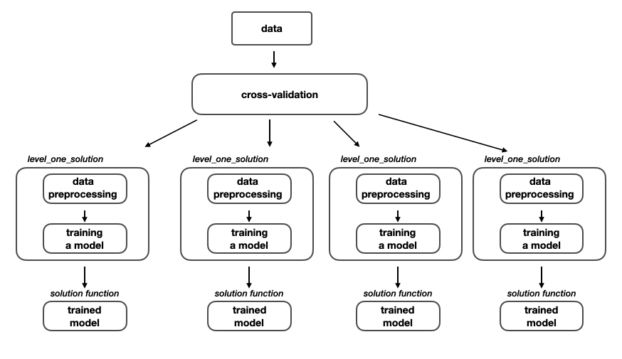Level one model training

After the execution of this pipeline we have 4 models that are capable of providing us a solution for the MoA competition. In fact we can submit each of them separately and check their performances. What is important here to note is that every model was trained with different preprocessing function, so whenever we want to make predictions with that model on new unseen data we need to pass the data to the model’s specific data preprocessing function.

In order our blending to be more successful at the end, our models need to be more diversified i.e less correlated. If we blend two almost identical models then we are not going to be getting any new information from the blend as it will be just like averaging a single model. On the other hand, if we blend models that have completely different view of the world, the final blended model will have a little bit of both worlds regarding which-one was more real. To make the models more diversified I used 4 different neural network architectures and 4 different data-scaling functions. The 4^th model which is a 1D-CNN was inspired by the beautiful explanaition of the solution that achieved second place on this competition.

As discussed before, I am using 5 fold cross-validation strategy so in every solution function I will end up with 5 different weights for the neural network used in that solution. Additionally, to make the predictions more stable and to reduce the randomness, I execute each solution function on 3 different seeds and in the end I average out the predictions of each seed.

Training the stacked model - level two

When we have successfully trained the 4 separate models, we can go one level further and train the stacked model. This training pipeline is almost identical with the previous one, there is just one additional detail that is creating new dataset based on the predictions obtained by the previous models.

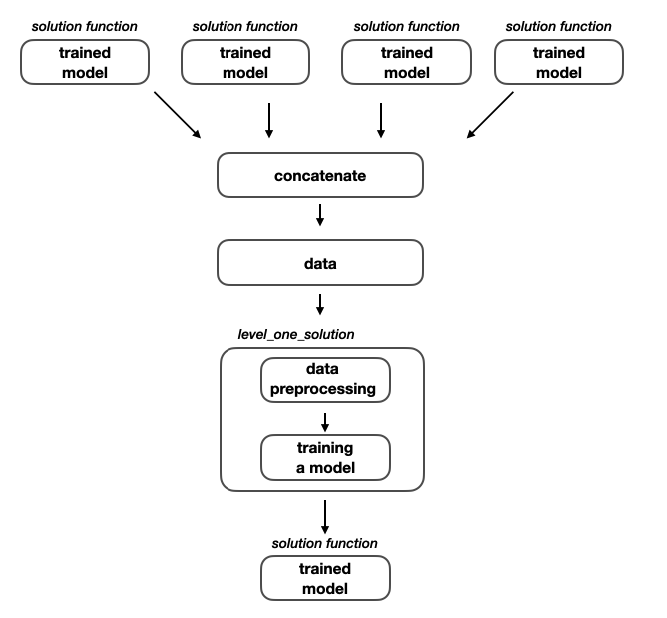Level two model training

This is the last model that is trained, so after this process has finished we end up with total of 5 trained models. The first 4 are level one models and can be directly submitted to the competition while the 5^th stacked model is dependent of the predictions of the previous models.

Final submission

The goal of the inference notebook is to load all of the previously trained neural networks where each network represents a solution function to the MoA competition problem. We saw in the previous section that after finishing with the whole training process we end up with 5 different trained models architectures. Since every model architecture was trained on 5 folds and every training process was executed on 3 different seeds, we end up with 15 saved weights for every one of the 5 models architectures. The predictions from those 15 neural networks for each model architecture are simply averaged and afterwards we end up with 5 different predictions which represents the total number of model used.

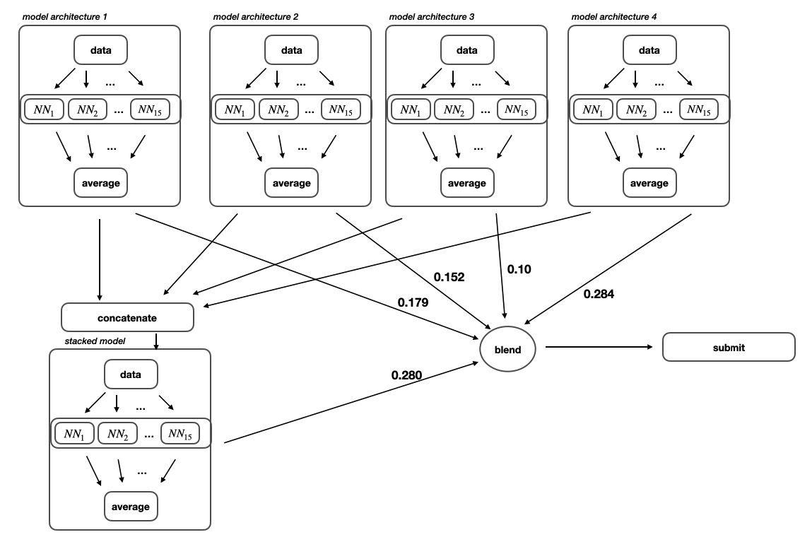Blendig weights of the trained models

There are multiple ways of blending the predictions of the 5 different models. One possible way is to submit the 4 level one models to the competition and then assign weights based on their performance on the public leaderboard. Another way is to decide if the target is activated based on majority vote of the multiple models. I decided to calculate the blend weights based on the best performance on my local validation score.

Final thoughts

Good job, you made it all the way to the end. I want to thank you very much for reading the blog post and I hope that you had a fun time and maybe learnt something new. This was my first writing experience of this kind, so any feedback is much appreciated.

I really enjoyed competing in this MoA competition on Kaggle and I am really thankful for all the people who made this competition possible. Looking forward for the next one and for the next blog post!